Low-cost air pollution monitors have many advantages, such as size and price. On the other hand, these monitors provide estimates for PM2.5 with higher uncertainties compared to expensive reference monitors. We are aware of these uncertainties, and hence, we have initiated a global co-location project, where we sent our Open Air outdoor monitors to more than 20 sites around the globe. Our invaluable local partners have set up these monitors next to their reference stations and made their reference data accessible to us. The comparison between the reference and Open Air data enables us to evaluate the accuracy of our monitors. Moreover, it allows us to implement correction algorithms to increase the accuracy of our raw readings. Although the co-location project is still ongoing, we now have several months of data that we can use to implement an algorithm.
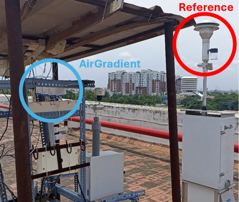
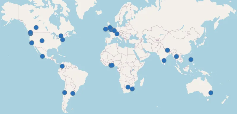
Below are two images. The picture on the left illustrates three of our monitors that are co-located with a reference station in Chennai, India. The map on the right indicates other sites in our co-location project.
How accurate are our Open Air PM2.5 readings?
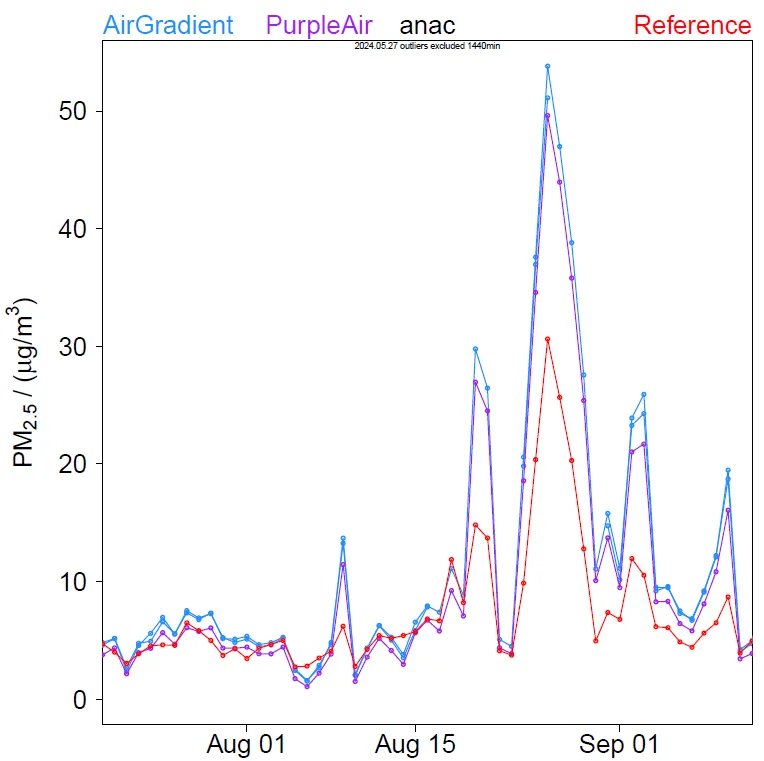
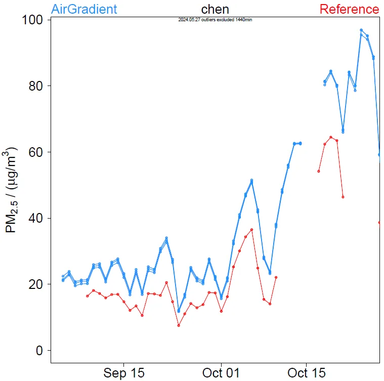
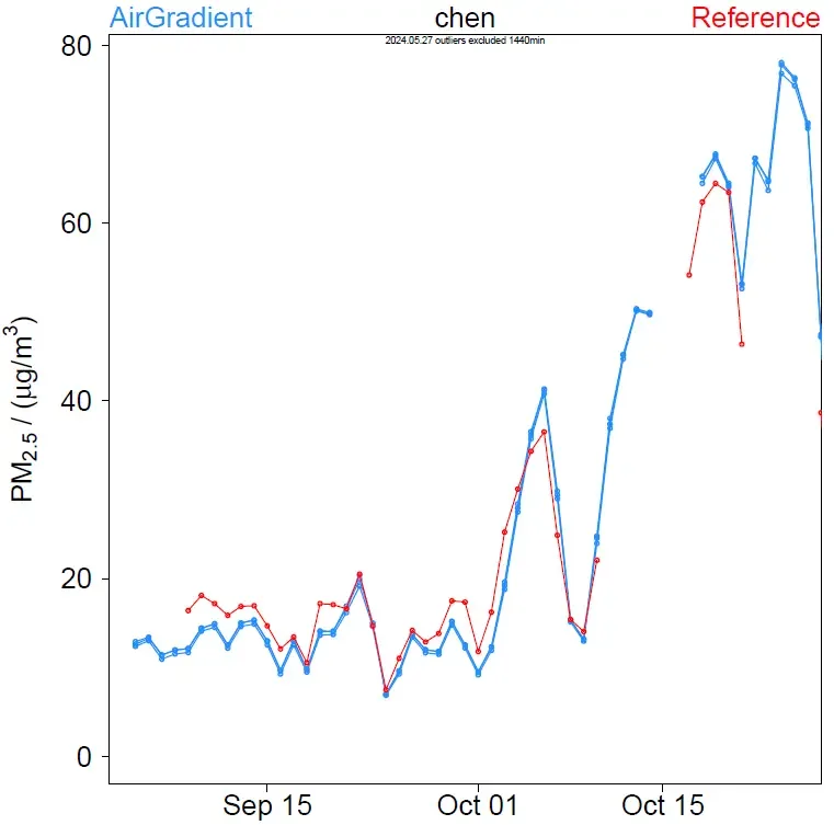
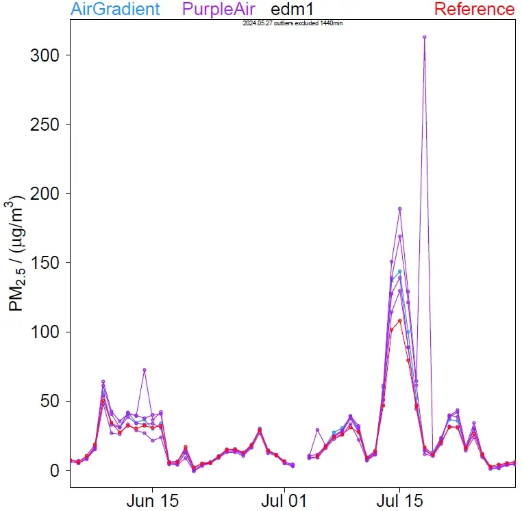
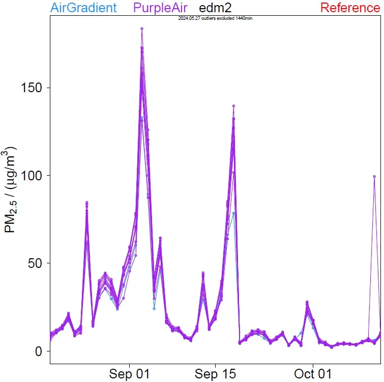
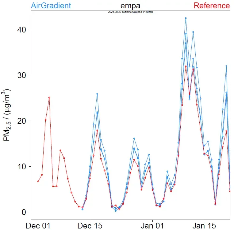
Before talking about correction, let’s talk about the raw readings. How accurate are they? The blue timelines in the plots below show the raw readings for PM2.5 from our Open Air monitors in 10 locations over a time period of 50 days. The red lines refer to the readings from the reference monitors, which can be considered of the highest accuracy. For comparison, some plots also include purple lines, which refer to raw data from low-cost outdoor monitors from PurpleAir. Most plots include multiple blue lines, as multiple Open Air monitors are available per location. All data points are daily averages.
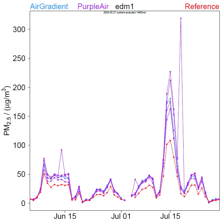
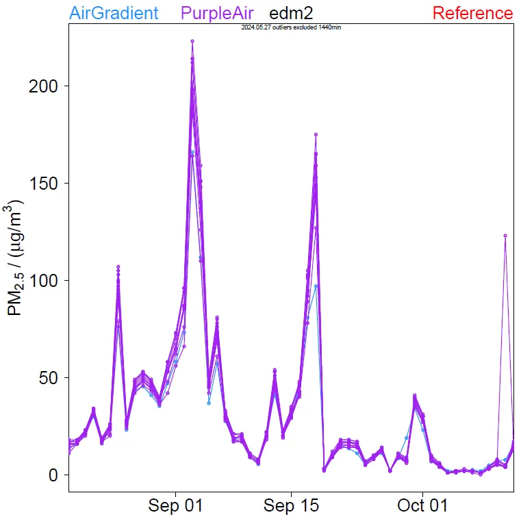
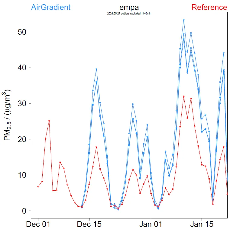
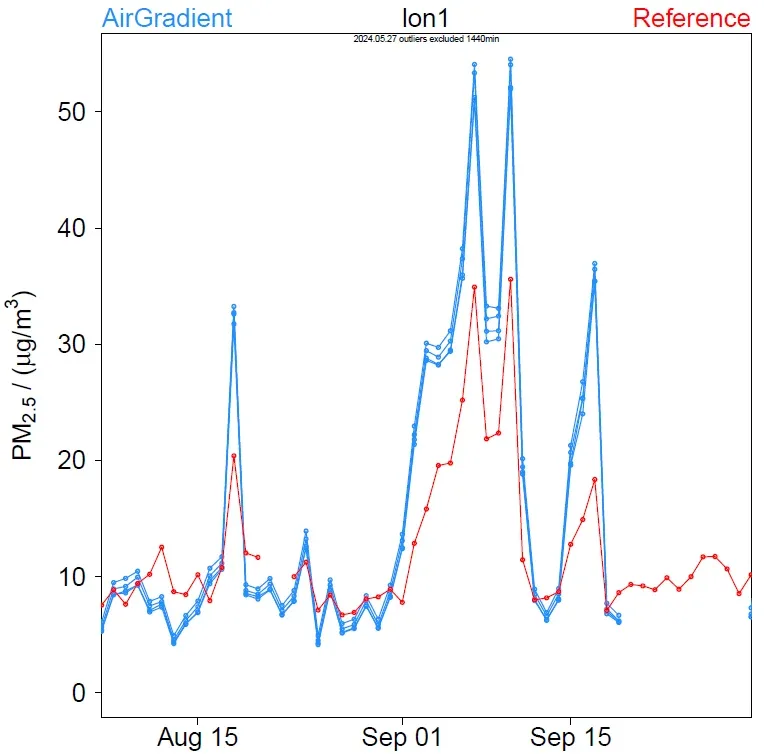
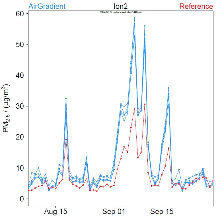
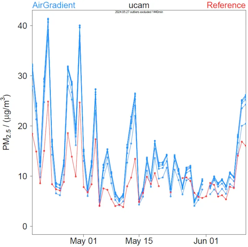
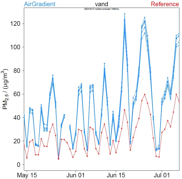
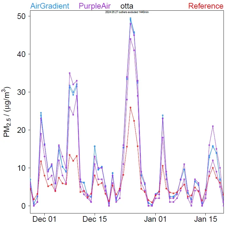
The table below provides information about the locations and reference instruments:
| Abbreviation | City | Country | Reference |
|---|---|---|---|
| anac | Anacortes | United States | BAM 1020 |
| chen | Chennai | India | BAM 1022 |
| edm1 | Edmonton (Greenwood) | Canada | Grimm 180 |
| edm2 | Edmonton (Eastgate) | Canada | No reference data available |
| empa | Dübendorf | Switzerland | Palas Fidas |
| lon1 | London (Marylebone Road) | United Kingdom | BAM |
| lon2 | London (Honor Oak Park) | United Kingdom | Palas Fidas 200E |
| ucam | Cambridge | United Kingdom | Palas Fidas 200S |
| vand | Vanderbijlpark | South Africa | Grimm |
| otta | Ottawa | Canada | Not disclosed |
Based on the plots above, it seems that different Open Air monitors at the same location report similar results, implying relatively high reproducibility. Additionally, it seems that the Open Air monitors overestimate PM2.5 in a systematic manner during periods with elevated PM2.5 concentrations. In contrast, they report rather low concentrations when PM2.5 pollution is very low. A similar behaviour is observed for the monitors from PurpleAir. This finding is unsurprising as both AirGradient and PurpleAir rely on optical particle counters from Plantower as a PM sensor. The exact reason for the inaccurate PM readings is unknown to us. However, given that Plantower’s PMS5003 is based on light scattering, it would be surprising if no systematic deviations were observed. Note that instruments based on light scattering measure PM2.5 with respect to optical diameters, whereas PM2.5 is generally defined as aerodynamic diameter. These are two different concepts that can only be directly compared upon conversion with shape factor, density and refractive index, which are generally unknown for ambient PM. Alternatively, one can be converted into another using an empirically derived correction algorithm, which will be the topic of the next section of this article.
PM2.5 correction algorithm
There is an already existing PM2.5 correction algorithm developed by scientists from the United States Environmental Protection Agency (EPA) based on outdoor monitors from PurpleAir in the context of wildfires. EPA uses this algorithm to correct raw PurpleAir data for the AirNow Fire and Smoke Map. The previous section of this blog revealed that the PM readings from AirGradient and PurpleAir are similar, hence, the question arises as to whether the algorithm from EPA is also applicable to AirGradient? As this algorithm is based on raw humidity readings from the low-cost monitor, we first need to understand if the humidity readings from AirGradient and PurpleAir are comparable. The plots below show daily averages of raw relative humidity data from AirGradient in blue, PurpleAir in purple and the reference in red.
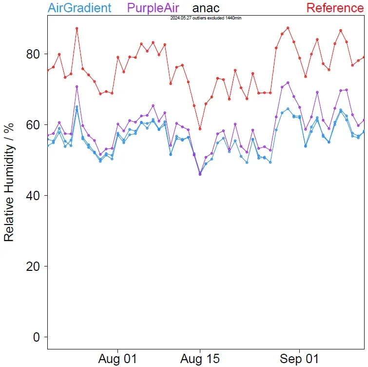
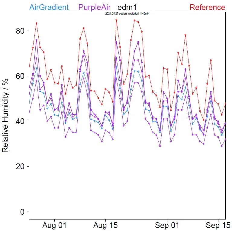
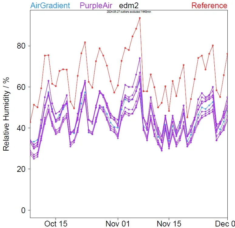
Based on the plots above, it appears that a potential systematic difference in humidity between AirGradient and PurpleAir is minor in comparison to the deviation within a set of PurpleAir monitors. In other words, there is no systematic difference between the humidity readings from AirGradient and PurpleAir based on the currently available data. In this case, let’s look at the correction algorithm from EPA, which can be found here (Eq. 4). It uses different corrections for different raw PM concentrations (PAcfatm). The variable ‘RHraw’ stands for raw relative humidity readings from the low-cost monitor. The formulas below were taken from the EPA PDF.
For raw readings below 30 µg/m³:
PM2.5 = [0.524 × PAcfatm] − [0.0862 × RHraw] + 5.75
For raw readings between 30 and 50 µg/m³:
PM2.5 = [0.786 × (PAcfatm/20 − 3/2) + 0.524 × (1 − (PAcfatm/20 − 3/2))] x PAcfatm − [0.0862 × RHraw] + 5.75
For raw readings between 50 and 210 µg/m³:
PM2.5 = [0.786 × PAcfatm] − [0.0862 × RHraw] + 5.75
For raw readings between 210 and 260 µg/m³:
PM2.5 = [0.69 × (PAcfatm/50 − 21/5) + 0.786 × (1 − (PAcfatm/50 − 21/5))] x PAcfatm− [0.0862 × RHraw × (1 − (PAcfatm/50 − 21/5))] + [2.966 × (PAcfatm/50 − 21/5)] + [5.75 × (1 − (PAcfatm/50 − 21/5))] + [8.84 × (10-4) × PAcfatm2 × (PAcfatm/50 − 21/5)]
For raw readings above 260 µg/m³:
PM2.5 = 2.966 + [0.69 × PAcfatm] + [8.84 × 10⁻⁴ × PAcfatm2 ]
According to EPA, this algorithm accounts for ‘bias and relative humidity at low concentration and the nonlinearity of PurpleAir response at higher concentration’. Let’s see how it performs with our AirGradient data. The plots below are a repetition of the previous plots, but this time, the AirGradient and PurpleAir time points are corrected with EPA’s algorithm.
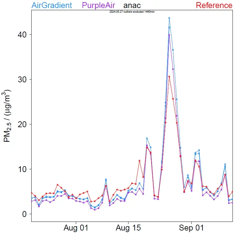
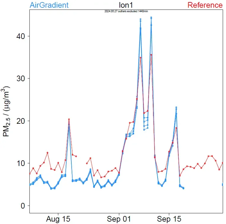
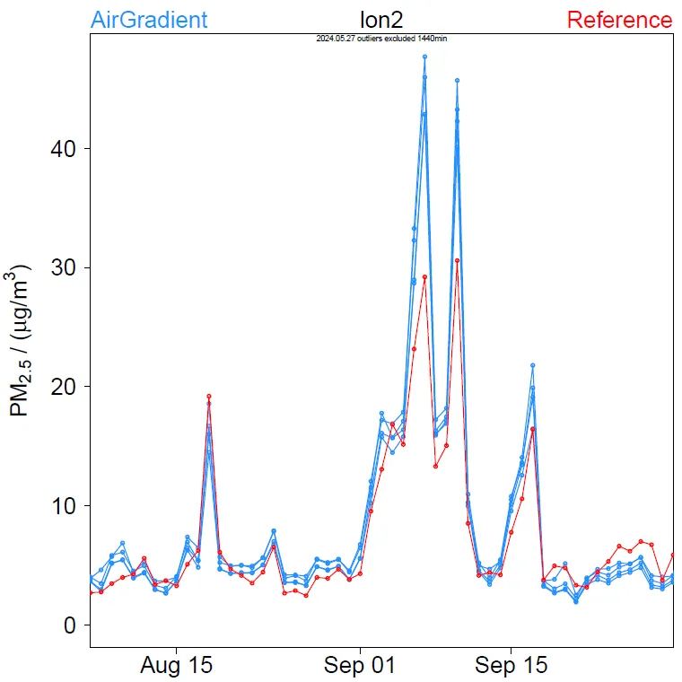
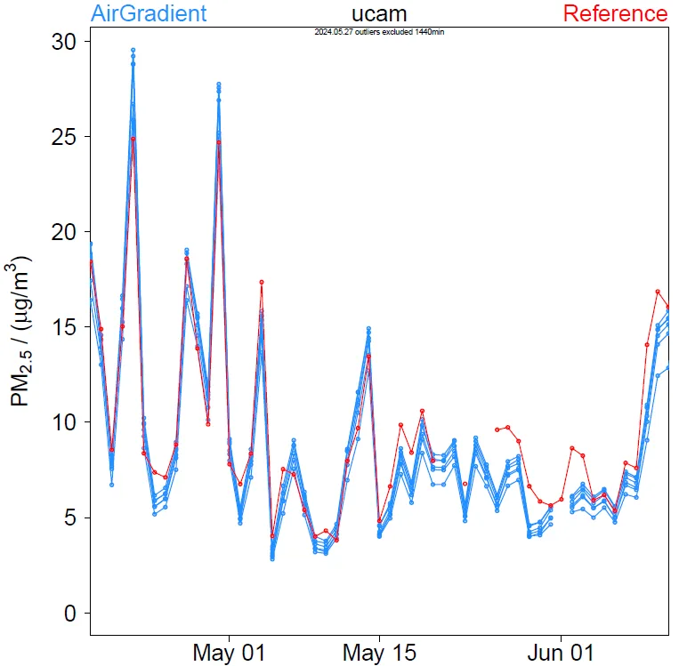
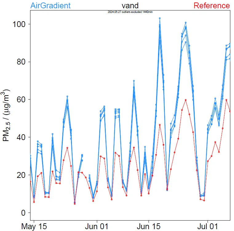
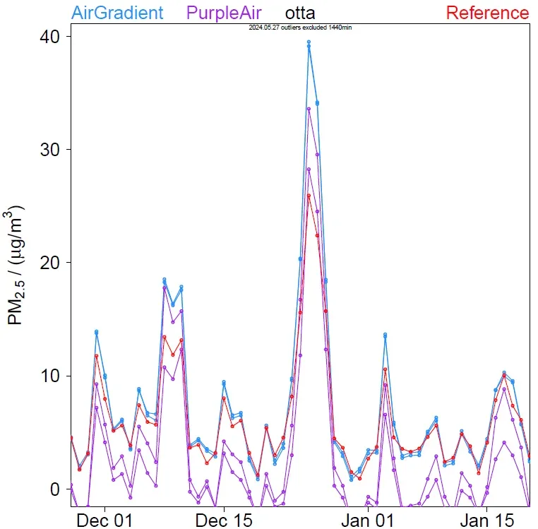
At first glance, the accuracy of both AirGradient and PurpleAir improves when the correction algorithm from EPA is applied. It makes sense to run some scatter plots to better determine the error of the sensors. The plots in the appendix show AirGradient data from individual locations in comparison to the reference (scatterplots, raw and corrected). A summary of the daily PM2.5 raw (left) and corrected data (right) from all locations is shown below, once with full scale and once with a subset from 0 to 50 µg/m³. The reference is situated on the y- and AirGradient Open Air on the x-axis.
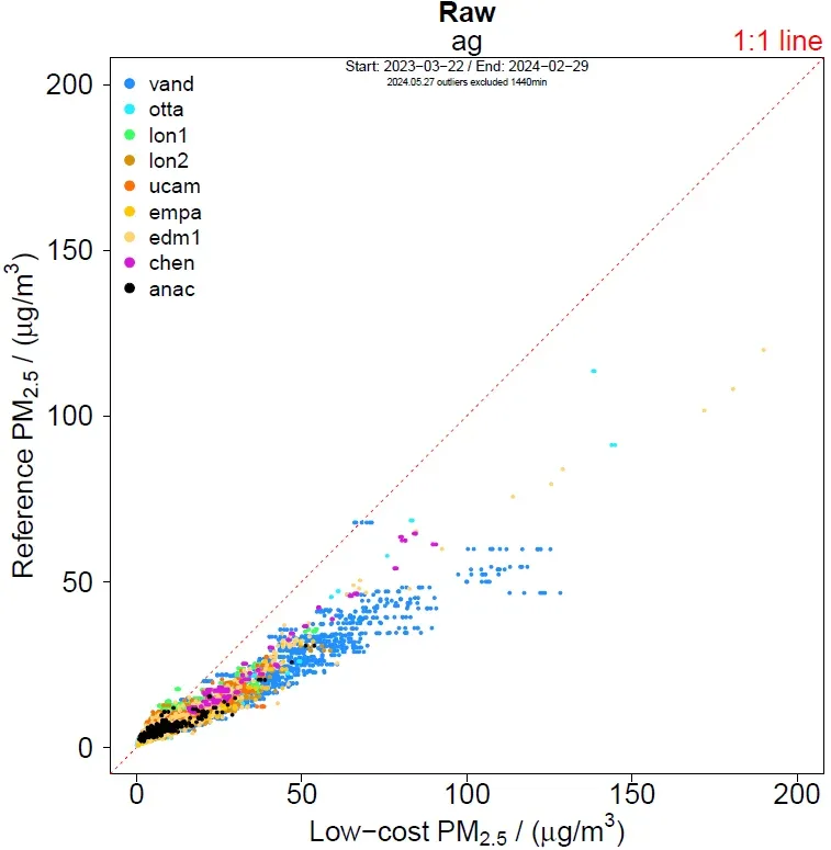
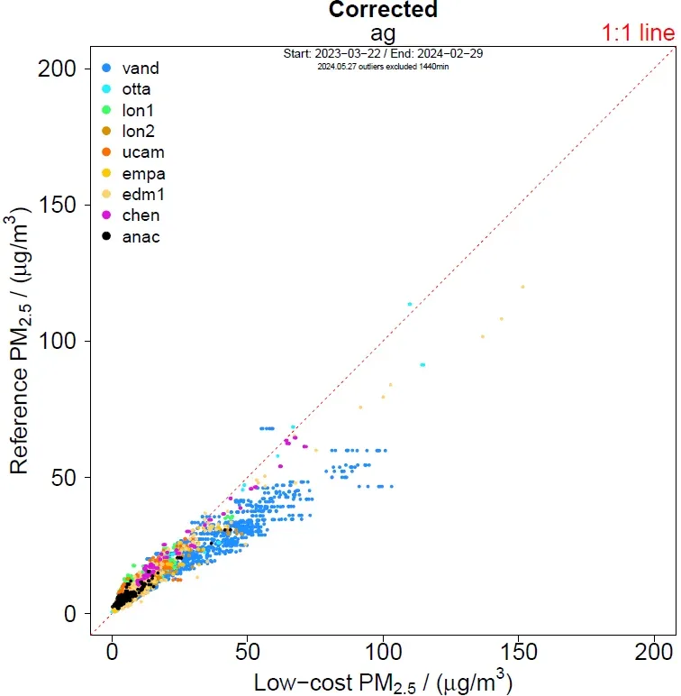
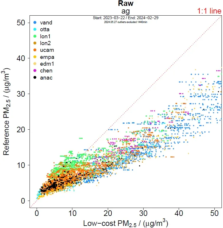
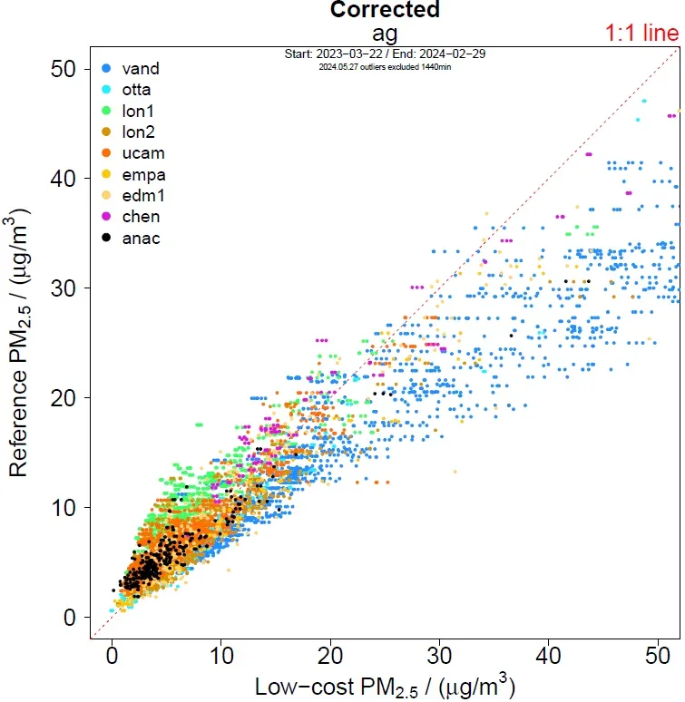
The readings of all locations seem to get closer to the 1:1 line when applying the correction, which is encouraging. When looking carefully, we see that not all locations improve to the same extent. The correction seems to be less accurate in Vanderbijlpark, South Africa (denoted as ‘vand’). Let's repeat the previous 4 scatter plots, but this time leave out this location to make the other locations more visible. We come back to Vanderbijlpark later in this blog article.
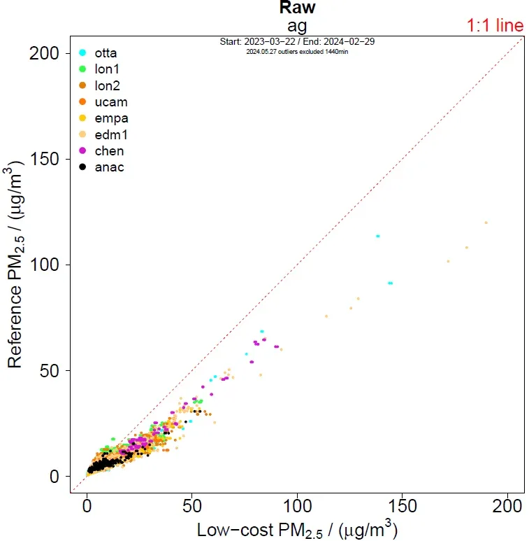
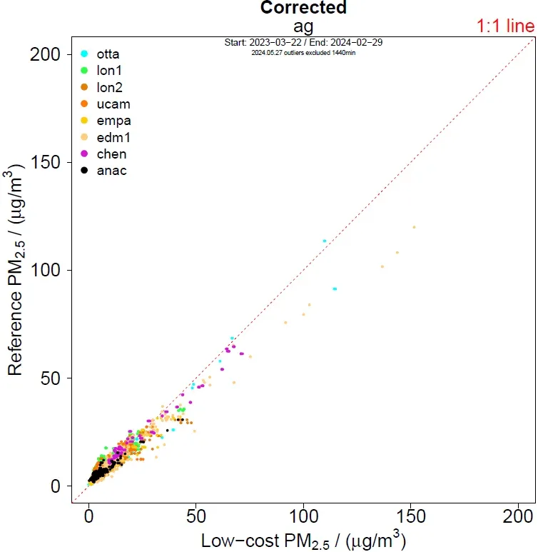
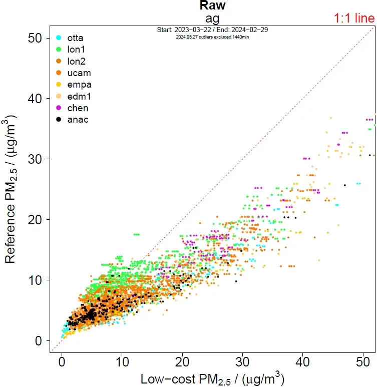
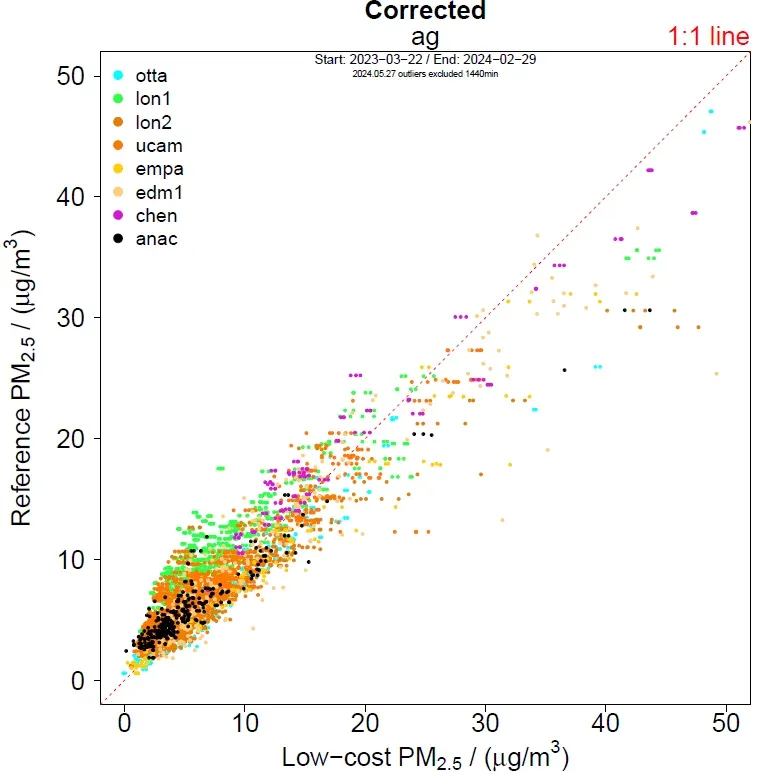
The table below provides a numerical overview of the scatter plots with raw and corrected AirGradient data. Our webinar about sensor accuracy explains what these variables mean and how to interpret them. More details (slope, intercept, MAE, RMSE and mean) are outlined in the appendix for individual locations as well as sensors.
| Location | N | R² Raw | R² Corrected | nRMSE Raw (%) | nRMSE Corrected (%) | nRMSE Improvement (factor) |
|---|---|---|---|---|---|---|
| Anacortes | 316 | 0.86 | 0.905 | 87 | 34 | 2.6 |
| Chennai | 150 | 0.97 | 0.98 | 52 | 15 | 3.5 |
| Edmonton 1 | 251 | 0.97 | 0.97 | 89 | 39 | 2.3 |
| Dübendorf (empa) | 138 | 0.933 | 0.977 | 120 | 32 | 3.8 |
| London 1 | 1056 | 0.815 | 0.857 | 47 | 34 | 1.4 |
| London 2 | 1050 | 0.85 | 0.86 | 96 | 36 | 2.7 |
| Ottawa | 481 | 0.93 | 0.97 | 103 | 29 | 3.6 |
| Cambridge (ucam) | 1668 | 0.868 | 0.888 | 74 | 26 | 2.8 |
| Vanderbijlpark | 1649 | 0.892 | 0.903 | 103 | 58 | 1.8 |
| Average | 0.899 | 0.923 | ~86 | ~34 | ~2.5 |
Using nRMSE as a metric, the accuracy of AirGradient’s Open Airs significantly improved when applying EPA’s correction algorithm. On average, the nRMSE, i.e. the relative error of the monitors, dropped to less than half compared to the error of the raw data. Note that all investigated locations showed improved accuracy, demonstrating that EPA's algorithm generally enhances the performance of AirGradient’s Open Air monitors.
Why does the data from Vanderbijlpark look different to the other locations?
As previously noted, the correction algorithm seems to be less effective in Vanderbijlpark (vand), South Africa. Readings for elevated PM2.5 levels of > 20 µg/m³ seem further away from the 1:1 line compared to other locations such as Chennai (chen), Ottawa (otta) or Edmonton (edm1), even when applying correction. This could be the result of different physical PM2.5 properties in that location. It could also be related to the reference instrument. Note that different reference instruments may use different measuring principles and may be calibrated differently. More data is currently being acquired to further investigate. Despite this phenomenon, the nRMSE in Vanderbijlpark also improves significantly when the correction algorithm is applied.
Indoor
Although the co-location project focuses on outdoor data, we also have some hourly indoor data from multiple AirGradient ONE’s that are co-located with a MODULAIR monitor from QuantAQ in Manchester, England. Note that this reference monitor is neither a Federal Reference Method (FRM) nor a Federal Equivalent Method (FEM). However, co-location of a MODULAIR monitor with research and/or regulatory-grade instruments has shown high correlation coefficients (R2 = 0.936) and low mean absolute errors (MAE = 1.2 µg/m³) for hourly PM2.5 data according to QuantAQ. The normalized MAE is unknown to us.
Timelines and scatter plots for the co-location of AirGradient One with QuantAQ MODULAIR are shown here:
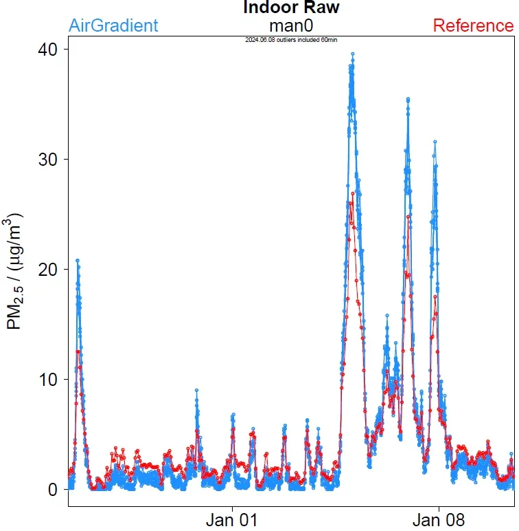
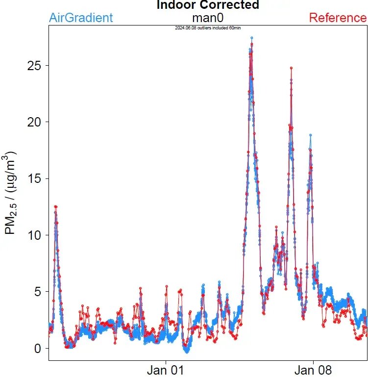
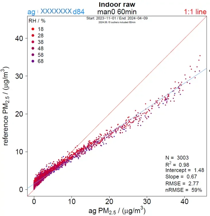
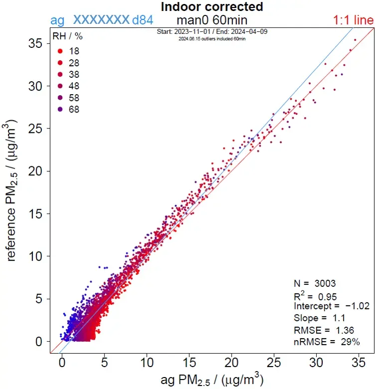
Based on the available data and nRMSE as a metric, it seems that the correction algorithm also improves the accuracy of the AirGradient indoor monitors (nRMSE improved from 59 % to 29 %).
Conclusion
The analysed outdoor data set comprised 6759 daily PM2.5 Open Air data points for which co-located reference data were available at 9 locations in 6 countries. That’s almost 20 years of co-located data. On average, the correction algorithm from EPA significantly improved the total nRMSE from 86 % to 34 %. Similarly, the nRMSE of the indoor monitors from one co-location improved from 59 % to 29 %. Although the algorithm does not seem to improve sensor performance in all locations in the same way, we have decided to implement it for multiple reasons: all analysed locations show improved average accuracy using nRMSE as a metric, we advocate using an already established algorithm to allow better comparability and uniformity between different brands, and there is no training bias as we did not use our own data to develop the model. Nevertheless, we see the potential for improvement in EPA’s correction algorithm. For example, it leads to negative PM2.5 concentrations when humidity is high, and the raw PM readings are low. See below on the left side a screenshot from PurpleAir’s map where negative PM2.5 concentrations are reported by a monitor in Monterey (California) according to EPA’s correction algorithm. Note that EPA on the Fire and Smoke Map seem to exclude negative concentrations from PurpleAir monitors, as shown in the screenshot below on the right side from the same sensor in Monterey.

Implementation
Implementing a correction algorithm poses a risk as it may introduce confusion. To provide clarification, we have created an overview of all our correction algorithms. It clarifies what data is raw and what data is corrected.
We implement EPA’s PM2.5 algorithm (Eq. 4) with two changes:
- According to EPA’s algorithm, a raw reading of 0 µg/m³ will result in a corrected PM2.5 concentration ranging from -2.9 to 5.8 µg/m³, depending on humidity. However, we interpret a raw reading of 0 µg/m³ differently, as we believe such a reading is below the detection limit of the particle counter. In consequence, we decided not to apply corrections for raw readings that are 0 µg/m³. Note that a raw reading of, for example, 0.1 µg/m³ will still be converted according to EPA’s algorithm.
- We believe negative PM2.5 levels are confusing, hence we decided to remove corrected values that are negative. Instead, we will display the value 0 µg/m³.
The Appendix can be downloaded here.
The data this article is based on can be found here.
A big thank you goes to everyone who supported this study by co-locating our sensors and providing reference data:
Sri Ramachandra Institute of Higher Education and Research (Deemed to be University), India
Swiss Federal Laboratories for Materials Science and Technology
Update
Since the release of this article, our colocation data has doubled. We have repeated the analysis in a second article, now covering 17 outdoor locations in 11 countries with 37 years of PM2.5 colocation data. The new results mostly confirmed what we saw before: the EPA formula really does improve the accuracy of Plantower sensors around the world. But it also brought up some interesting new insights — like how the type of reference instrument you use can actually affect the results of the accuracy analysis. Take a look!
